import numpy as np
import scipy.linalg as sla
import scipy.sparse as sparse

import matplotlib.pyplot as plt
%matplotlib inline

Topology design optimization

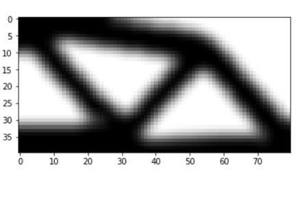
When performing optimization of structural problem, for example to obtain the bridge design above, you may want to use a numerical method called Finite Element Method. The optimization will consist of a series of solve of the form: $$ {\bf K} {\bf u} = {\bf F} $$

Here will load the matrix $ {\bf K}$ from a file. The matrix is given in Compressed Sparse Column (CSC) format.

K = sparse.load_npz('yourmatrix.npz')
K

K.shape[0]**2/105912

We can spy the distribution of the non-zero entries of the matrix:

plt.spy(K)
plt.show()

The matrix ${\bf K}$ has a banded format, and it is also symmetric and positive definite.

Kdense = K.todense()

np.max(Kdense-Kdense.T)

sla.norm(Kdense-Kdense.T)

Solving the linear system of equations using different methods:

F = np.zeros(K.shape[0])
F[1]=-1

LU factorization

u1 = sla.solve(Kdense,F)
u1.shape

%timeit sla.solve(Kdense,F)

lu,p = sla.lu_factor(Kdense)
u2 = sla.lu_solve((lu,p),F)
u2.shape

%timeit sla.lu_factor(Kdense)
%timeit sla.lu_solve((lu,p),F)

Cholesky factorization

Kcho = sla.cholesky(Kdense)
u3 = sla.cho_solve((Kcho,False),F)
u3.shape

%timeit sla.cholesky(Kdense)
%timeit sla.cho_solve((Kcho,False),F)

Sparse solve

from scipy.sparse.linalg import spsolve

u4 = spsolve(K,F)
u4.shape

%timeit spsolve(K,F)